Found in a list of 100+ interesting data sets, the Texas Department of Criminal Justice provides different collections of information on death row inmates both present and past. Prior occupations for each current offender are listed here.

Dependencies

We’ll need some packages to scrape, cluster, and chart our findings.

rvest: “Wrappers around the ‘xml2’ and ‘httr’ packages to make it easy to download, then manipulate, HTML and XML.”
wordcloud: “Pretty word clouds.”
tm: “A framework for text mining applications within R.”
apcluster: “The ‘apcluster’ package implements Frey’s and Dueck’s Affinity Propagation clustering in R.”

library(rvest)
library(wordcloud)
library(tm)
library(apcluster)

Collection

The data we wish to look at is not in the form we need it. We’ll need to capture the HTML and parse it looking for the prior occupation information. Using rvest, we will grep for all <p> tags that contain the occupation information. Not every page is consistent so we will need some logic to hunt around for the prior occupation field. Once we’ve parsed every page, all of the raw information will be saved to a CSV file for later pre-processing. Each line corresponds to each death row inmate prior occupations collected.

# -----------------------
# Scraping
# -----------------------

base_link <- 'https://www.tdcj.state.tx.us/death_row/'
main_link <- 'https://www.tdcj.state.tx.us/death_row/dr_offenders_on_dr.html'
csv_filename <- 'prior_occupations_dirty.csv'

if (!file.exists(csv_filename)) {
  page <- read_html(main_link)
  page
  links <- html_attr(html_nodes(page, 'a'), 'href')
  links
  links <- grep('^dr_info.*html$', links, value=TRUE)
  links
  prior_occupations_dirty <- c()
  for (link in links) {
    texts <- read_html(paste(base_link, link, sep='')) %>% html_nodes('p') %>% html_text()
    if (length(grep('Prior Prison', texts[3])) >= 1) {
      prior_occupations_dirty <- c(prior_occupations_dirty, texts[2])
    } else {
      prior_occupations_dirty <- c(prior_occupations_dirty, texts[3])
    }
  }
  prior_occupations_dirty_df = as.data.frame(prior_occupations_dirty)
  write.csv(prior_occupations_dirty_df, file=csv_filename)
}

Pre-processing

With the CSV file opened, we need to clean each entry for unwanted white-space and punctuation. For those with multiple prior occupations, we’ll split on the commas. Once cleaned, we’ll add each prior occupation per inmate to the inmates_occupations list.

# -----------------------
# Cleaning
# -----------------------

csv_file <- read.csv(file=csv_filename)
prior_occupations_dirty <- as.vector(t(csv_file$prior_occupations_dirty))

prior_occupations_cleaned = c()
inmates_prior_occupations = list()
i <- 1
for (prior_occupation_dirty in prior_occupations_dirty) {
  prior_occupation <- gsub('Prior Occupation', '', prior_occupation_dirty)
  prior_occupation <- tolower(prior_occupation)
  prior_occupation <- gsub('^\\W+|^\\s+', ' ', prior_occupation)
  prior_occupation <- gsub('`', '', prior_occupation)
  prior_occupation <- gsub(':', ' ', prior_occupation)
  prior_occupation <- gsub('\\.', ' ', prior_occupation)
  prior_occupation <- gsub('\r', ' ', prior_occupation)
  prior_occupation <- gsub('\n', ' ', prior_occupation)
  prior_occupation <- gsub('\\s+', ' ', prior_occupation)
  if (length(grep('n/a', prior_occupation)) == 0) {
    prior_occupation <- gsub('/', ', ', prior_occupation)
  }
  prior_occupation <- gsub(' and ', ', ', prior_occupation)
  prior_occupation <- gsub('&', ', ', prior_occupation)
  prior_occupation <- gsub(';', ', ', prior_occupation)
  prior_occupation <- trimws(prior_occupation)
  prior_occupations <- strsplit(prior_occupation, ', ')
  prior_occupations <- lapply(prior_occupations, function (x) return(gsub('\\s+', ' ', x)))
  prior_occupations <- lapply(prior_occupations, function (x) return(trimws(x)))
  if (length(prior_occupations[[1]]) > 0) {
    prior_occupations_cleaned <- c(prior_occupations_cleaned, prior_occupations, recursive=T)
    inmates_prior_occupations[[toString(i)]] <- prior_occupations[[1]]
    i <- i + 1
  }
}
total_inmate_count = length(inmates_prior_occupations)

Looking over the dataset, you’ll notice some redundancies such as mechanic versus auto mechanic. With care, we will condense the prior occupations to the sub-strings of the redundancies. We’ll also need to hard-code some corrections for irregularities such as fork lift versus forklift. Once the duplicates have been merged, we’ll generate a unique list of the prior occupations for our axis labels.

# -----------------------
# Duplication Removal
# -----------------------

prior_occupations_merged = c()
prior_occupations_merged_map = list()
for (prior_occupation_cleaned1 in prior_occupations_cleaned) {
  prior_occupation <- prior_occupation_cleaned1
  if (is.null(prior_occupations_merged_map[[prior_occupation]])) {
    if (nchar(prior_occupation) >= 4) {
      for (prior_occupation_cleaned2 in prior_occupations_cleaned) {
        if (nchar(prior_occupation_cleaned2) >= 4) {
          if (length(grep(prior_occupation_cleaned2, prior_occupation)) > 0) {
            if (nchar(prior_occupation) >= nchar(prior_occupation_cleaned2)) {
              prior_occupation <- prior_occupation_cleaned2
            }
          }
        }
      }
    }
    if (prior_occupation == 'n/a') {
      prior_occupation <- 'none'
    }
    if (length(grep('air condition', prior_occupation)) > 0) {
      prior_occupation <- 'ac'
    }
    if (length(grep('fork lift', prior_occupation)) > 0) {
      prior_occupation <- 'forklift'
    }
    if (length(grep('forklift', prior_occupation)) > 0) {
      prior_occupation <- 'forklift'
    }
    if (length(grep('clerical', prior_occupation)) > 0) {
      prior_occupation <- 'clerk'
    }
    if (length(grep('welding', prior_occupation)) > 0) {
      prior_occupation <- 'welder'
    }
    prior_occupations_merged_map[[prior_occupation_cleaned1]] <- prior_occupation
  } else {
    prior_occupation <- prior_occupations_merged_map[[prior_occupation]]
  }
  prior_occupations_merged <- c(prior_occupations_merged, prior_occupation)
}
total_prior_occupation_count = length(prior_occupations_merged)

i <- 1
for (inmate_prior_occupations in inmates_prior_occupations) {
  temp = c()
  for (prior_occupation in inmate_prior_occupations) {
    temp <- c(temp, prior_occupations_merged_map[[prior_occupation]])
  }
  inmates_prior_occupations[[toString(i)]] <- temp
  i <- i + 1
}
unique_prior_occupations = unique(sort(prior_occupations_merged))
unique_prior_occupations_length <- length(unique_prior_occupations)

Mining

We have collected, cleaned, and removed erroneous variations in our dataset. Now we’ll move on to mining and plotting/charting our data.

Total Prior Occupation Relative Frequency Distribution

Let us begin by charting the relative frequency of prior occupations listed across all sampled inmates.

# -----------------------
# Prior Occupation Relative Frequency Chart
# -----------------------

reverse_table <- function(t) { t[sort(names(t), decreasing=T)] }

prior_occupations_table <- reverse_table(table(prior_occupations_merged))
prior_occupations_table <- prior_occupations_table / sum(prior_occupations_table) * 100
png(file='prior_occupation_relative_freq_dist.png', width=1500, height=1500)
par(
  mai=c(2.0, 3.0, 1.0, 1.0)
)
barplot(
  prior_occupations_table,
  horiz=T,
  col=rainbow(length(prior_occupations_table)),
  cex.names=1.1,
  las=1,
  xlim=c(0, 100),
  axes=T,
  border=NA
)
axis(1, at=seq(0,100,5))
grid(nx=100, ny=NA)
barplot(
  prior_occupations_table,
  horiz=T,
  col=rainbow(length(prior_occupations_table)),
  cex.names=1.1,
  border=NA,
  las=1,
  xlim=c(0, 100),
  axes=T,
  add=T,
  xlab=paste('Percentage of', total_prior_occupation_count, 'listed Prior Occupations'),
  main=paste('Prior Occupation Relative Frequency Distribution of', total_inmate_count, 'Texas Death Row Inmates')
)
mtext('Prior Occupation', side=2, line=13)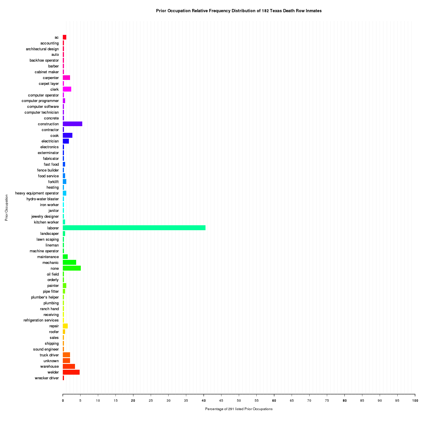

Prior Occupation Relative Frequency Distribution of 182 Texas Death Row Inmates

The unique prior occupations are in alphabetical order along the x-axis. The y-axis is the relative frequency distribution. laborer accounts for nearly 41% of the 291 listed prior occupations among the 182 death row inmates sampled. Attributing to its large percentage was the merging of duplicates, for example, general laborer and assembly line laborer into just laborer. One could argue that they are distinct labels. contruction and none are the second and third largest respectively.

We can explore the dataset further by clustering the sampled inmates by the prior occupations they had. We’ll treat each inmate as a document with their prior occupations making up the document. By clustering the inmates via their prior occupations, we can partition the dataset into different prior occupation profiles.

Inmate Prior Occupations Matrix

To begin clustering, we will need to vectorize each inmates’ prior occupations. We’ll assemble these vectors, into the inmate_matrix_count where [i][j] is >= 1 if the i^th inmate had the j^th occupation and 0 otherwise. No inmate had the same prior occupation listed more than once, so no count will be greater than one.

# -----------------------
# Inmate x Prior Occupations
# -----------------------

inmate_matrix_count <- c()
for (row in 1:length(inmates_prior_occupations)) {
  inmate_prior_occupations <- inmates_prior_occupations[[toString(row)]]
  for (unique_prior_occupation in unique_prior_occupations) {
    inmate_matrix_count <- c(
      inmate_matrix_count,
      sum(unique_prior_occupation == inmate_prior_occupations)
    )
  }
}
inmate_matrix_count = matrix(
  inmate_matrix_count,
  nrow=total_inmate_count,
  ncol=unique_prior_occupations_length,
  byrow=T
)

Prior Occupation Weighting (TF-IDF)

Since we are dealing with text and that nearly half of all sampled inmates were a laborer at some point, we’ll perform a term weighting technique known as TF-IDF. Given that an inmate was both a laborer and welder at some point, TF-IDF will weight laborer less since welder appears less frequently in the text corpus. Knowing that an inmate was a laborer does not say as much as knowing they were also a welder.

# -----------------------
# TF-IDF
# -----------------------

inmate_matrix_tfidf <- matrix(
  c(
    1:(total_inmate_count * unique_prior_occupations_length)
  ) * 0,
  nrow=total_inmate_count,
  ncol=unique_prior_occupations_length,
  byrow=T
)
nrow_count <- nrow(inmate_matrix_count)
for (row in 1:nrow(inmate_matrix_count)) {
  for (col in 1:ncol(inmate_matrix_count)) {
    tf <- inmate_matrix_count[row,col]
    df <- length(which(inmate_matrix_count[,col] > 0))
    idf <- log(nrow_count / (df + 1))
    tfidf <- tf * idf
    inmate_matrix_tfidf[row,col] <- tfidf
  }
}

Multidimensional Scaling (MDS)

To visualize the inmate vectors in two dimensions we’ll employ multidimensional scaling.

An MDS algorithm aims to place each object in N-dimensional space such that the between-object distances are preserved as well as possible.
Multidimensional Scaling, Wikipedia, the free encyclopedia

# -----------------------
# MDS
# -----------------------

plot_scale <- 1.0

scatter_plot_matrix <- function(prefix, input_matrix) {
  png(file=paste(tolower(prefix), 'scatter_plot.png', sep='_'), width=1500, height=1500)
  plot.new()
  input_matrix[,1]
  input_matrix[,2]
  textplot(
    input_matrix[, 1],
    input_matrix[, 2],
    seq(1:length(input_matrix[,1])),
    xlim=c(
      min(input_matrix[, 1]) * plot_scale,
      max(input_matrix[, 1]) * plot_scale
    ),
    ylim=c(
      min(input_matrix[, 2]) * plot_scale,
      max(input_matrix[, 2]) * plot_scale
    ),
    main=paste('Inmate Prior Occupations 2D Visualization', paste0('(', prefix, ')'))
  )
}

dist_matrix <- dist(inmate_matrix_count, method='euclidean')
inmate_matrix_count_mds <- cmdscale(dist_matrix)
scatter_plot_matrix('COUNT-MDS', inmate_matrix_count_mds)

dist_matrix <- dist(inmate_matrix_tfidf, method='euclidean')
inmate_matrix_tfidf_mds <- cmdscale(dist_matrix)
scatter_plot_matrix('TFIDF-MDS', inmate_matrix_tfidf_mds)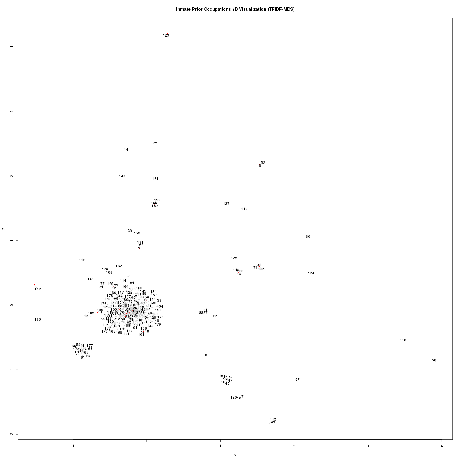

Inmate Prior Occupation 2D Visualization (TFIDF-MDS)

We can see a large mass around the origin. Another distinct mass is seen at (-0.8951273 -0.702121).

Affinity Propagation (AP) Clustering

Due to the concave shapes and variable density of the MDS scatter plot, we’ll employ Affinity Propagation Clustering. This has the added benefit of not having to specify the amount of clusters ahead of time (K).

# -----------------------
# AP CLUSTERING
# -----------------------

cluster_matrix <- function(prefix, input_matrix, inmates_prior_occupations) {
  apresult <- apcluster(negDistMat(r=2), input_matrix)
  input_cluster_labels = labels(apresult, type='enum')

  inmate_clusters_flt <- list()
  inmate_clusters_str <- list()

  i <- 1
  for (input_cluster_label in input_cluster_labels) {
    input_cluster_label <- toString(input_cluster_label)

    if (is.null(inmate_clusters_flt[[input_cluster_label]])) {
      inmate_clusters_flt[[input_cluster_label]] <- c()
      inmate_clusters_str[[input_cluster_label]] <- list()
    }

    inmate_clusters_flt[[input_cluster_label]] <- c(
      inmate_clusters_flt[[input_cluster_label]],
      input_matrix[i,]
    )

    i_str <- toString(i)
    temp = list()
    temp[[i_str]] <- inmates_prior_occupations[[i_str]]
    inmate_clusters_str[[input_cluster_label]] <- append(
      inmate_clusters_str[[input_cluster_label]],
      temp
    )

    i <- i + 1
  }

  for (cluster_i in 1:length(inmate_clusters_flt)) {
    cluster_i_str <- toString(cluster_i)
    cluster <- matrix(inmate_clusters_flt[[cluster_i_str]], ncol=2, byrow=T)
    inmate_clusters_flt[[cluster_i_str]] <- cluster
  }

  inmate_clusters_colors = rainbow(length(inmate_clusters_flt), v=0.8, s=0.5)

  write(
    sapply(
      sort(as.integer(names(inmate_clusters_str))),
      function(x) paste(
        'Cluster',
        toString(x),
        '\n ',
        paste('Inmate', names(inmate_clusters_str[[toString(x)]]), inmate_clusters_str[[toString(x)]], collapse='\n  ')
      )),
    paste(tolower(prefix), 'inmate_clusters.txt', sep='_')
  )

  return(list(flt=inmate_clusters_flt, str=inmate_clusters_str, colors=inmate_clusters_colors, labels=input_cluster_labels))
}

result <- cluster_matrix('TFIDF-MDS-AP', inmate_matrix_tfidf_mds, inmates_prior_occupations)
inmate_clusters_flt <- result$flt
inmate_clusters_str <- result$str
inmate_clusters_colors <- result$colors
inmate_cluster_labels <- result$labels

With the inmate_matrix_tfidf_mds clustered, we can now plot the clusters.

plot_clustering <- function(prefix, input_matrix, inmate_cluster_flt, inmate_clusters_colors, inmate_cluster_labels) {
  png(file=paste(tolower(prefix), 'inmate_clusters.png', sep='_'), width=1500, height=1500)
  plot.new()
  plot(
    input_matrix[,1],
    input_matrix[,2],
    main=paste('Death Row Inmate Clustering by Prior Occupations', paste0('(', prefix, ')'))
  )
  for (cluster_i in 1:length(inmate_clusters_flt)) {
    cluster_i_str <- toString(cluster_i)
    points(
      inmate_clusters_flt[[cluster_i_str]],
      col=inmate_clusters_colors[cluster_i],
      bg=inmate_clusters_colors[cluster_i],
      pch=19,
      cex=5,
      lwd=2
    )
  }
  text(
    input_matrix[, 1],
    input_matrix[, 2],
    inmate_cluster_labels,
    xlim=c(
      min(input_matrix[, 1]) * plot_scale,
      max(input_matrix[, 1]) * plot_scale
    ),
    ylim=c(
      min(input_matrix[, 2]) * plot_scale,
      max(input_matrix[, 2]) * plot_scale
    ),
  )
  legend(
    'topright',
    legend=lapply(c(1:length(inmate_clusters_colors)), function (x) return(toString(x))),
    fill=inmate_clusters_colors,
    cex=1.3,
    pt.cex=1
  )
}

plot_clustering('TFIDF-MDS-AP', inmate_matrix_tfidf_mds, inmate_clusters_flt, inmate_clusters_colors, inmate_cluster_labels)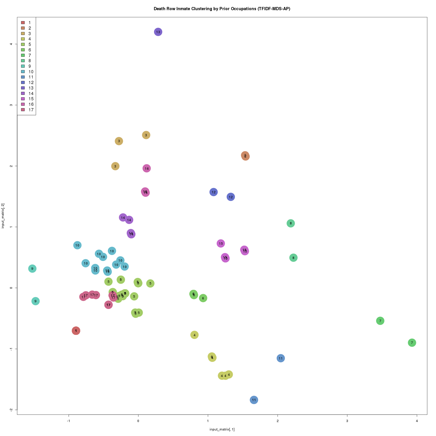

Death Row Inmate Clustering by Prior Occupations (TFIDF-MDS-AP)

In total, the algorithm generated 17 clusters. Cluster membership sizes range from one to 92 inmates.

Inmate Clusters, Prior Occupations Relative Frequency Distributions

Now let us generate a relative frequency distribution bar-chart for each TF-IDF MDS AP cluster.

plot_clusters_occupation_distributions <- function(prefix, inmate_clusters_str, unique_prior_occupations) {
  for (i in 1:length(inmate_clusters_str)) {
    cluster <- inmate_clusters_str[[toString(i)]]
    cluster_prior_occupations <- c()
    for (inmate_prior_occupations in cluster) {
      cluster_prior_occupations <- c(cluster_prior_occupations, inmate_prior_occupations)
    }

    prior_occupations_table <- reverse_table(table(factor(cluster_prior_occupations, levels=unique_prior_occupations)))
    prior_occupations_table <- prior_occupations_table / sum(prior_occupations_table) * 100

    png(file=paste(tolower(prefix), toString(i), 'prior_occupation_distribution.png', sep='_'), width=1500, height=1500)
    plot.new()
    par(
      mai=c(2.0, 3.0, 1.0, 1.0)
    )
    barplot(
      prior_occupations_table,
      horiz=T,
      col=rainbow(length(prior_occupations_table)),
      cex.names=1.1,
      las=1,
      xlim=c(0, 100),
      axes=T,
      border=NA
    )
    axis(1, at=seq(0,100,5))
    grid(nx=100, ny=NA)
    barplot(
      prior_occupations_table,
      horiz=T,
      col=rainbow(length(prior_occupations_table)),
      cex.names=1.1,
      las=1,
      xlim=c(0, 100),
      axes=T,
      add=T,
      ylab='',
      xlab=paste('Percentage of', length(cluster_prior_occupations), 'listed Prior Occupations'),
      main=paste(
        'Prior Occupation Relative Frequency Distribution of',
        length(cluster),
        'Texas Death Row Inmate(s) for Cluster',
        toString(i),
        paste0(
          '(',
          prefix,
          ')'
        )
      ),
      border=NA
    )
    mtext('Prior Occupation', side=2, line=13)
    dev.off()
  }
}

plot_clusters_occupation_distributions('TFIDF-MDS-AP', inmate_clusters_str, unique_prior_occupations)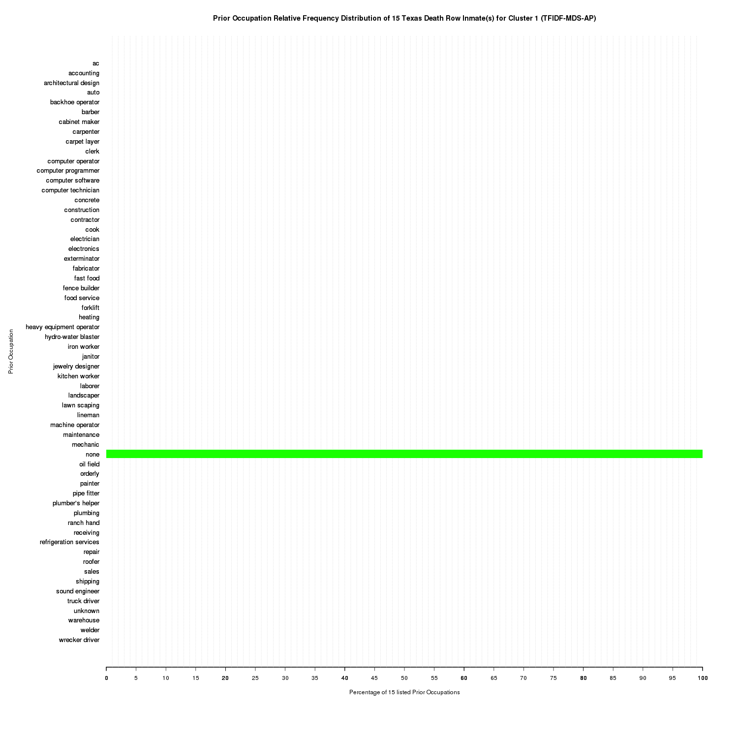

Prior Occupation Relative Frequency Distribution of 15 Texas Death Row Inmate(s) for Cluster 1 (TFIDF-MDS-AP)

Cluster 1, seen at (-0.8951273 -0.702121), is solely comprised of none which agrees with the dataset. Intuitively, if an inmate had no prior occupations, you wouldn’t expect to see other prior occupation terms clustered with none.

The following bar-charts are the clusters making up the large mass centered around the origin.

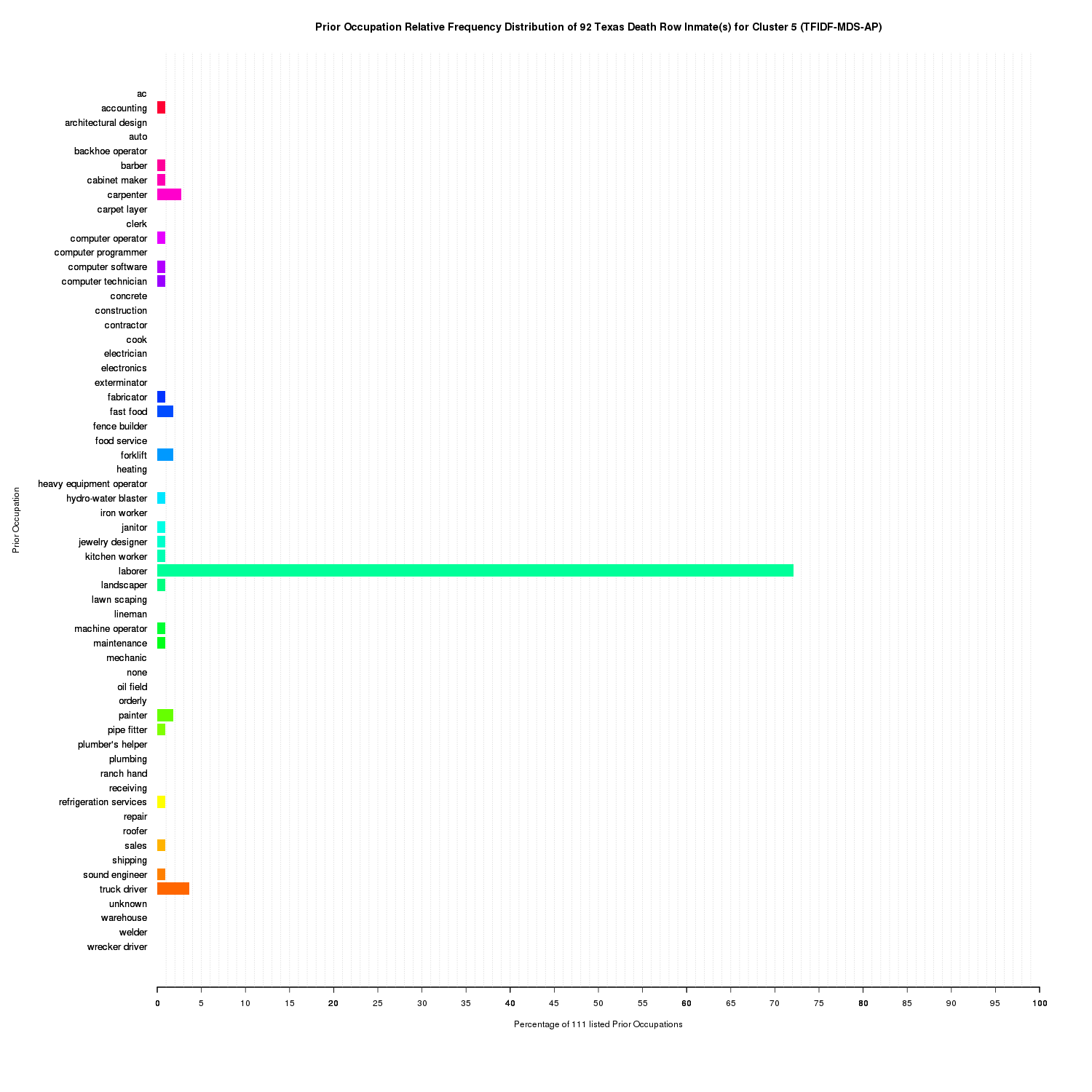
Prior Occupation Relative Frequency Distribution of 92 Texas Death Row Inmate(s) for Cluster 5 (TFIDF-MDS-AP)

Cluster 5 accounts for the inmates that were mainly laborers with only a very few having one other prior occupation. This cluster also contains a large portion of the unique prior occupations found in the raw data set such as computer software.

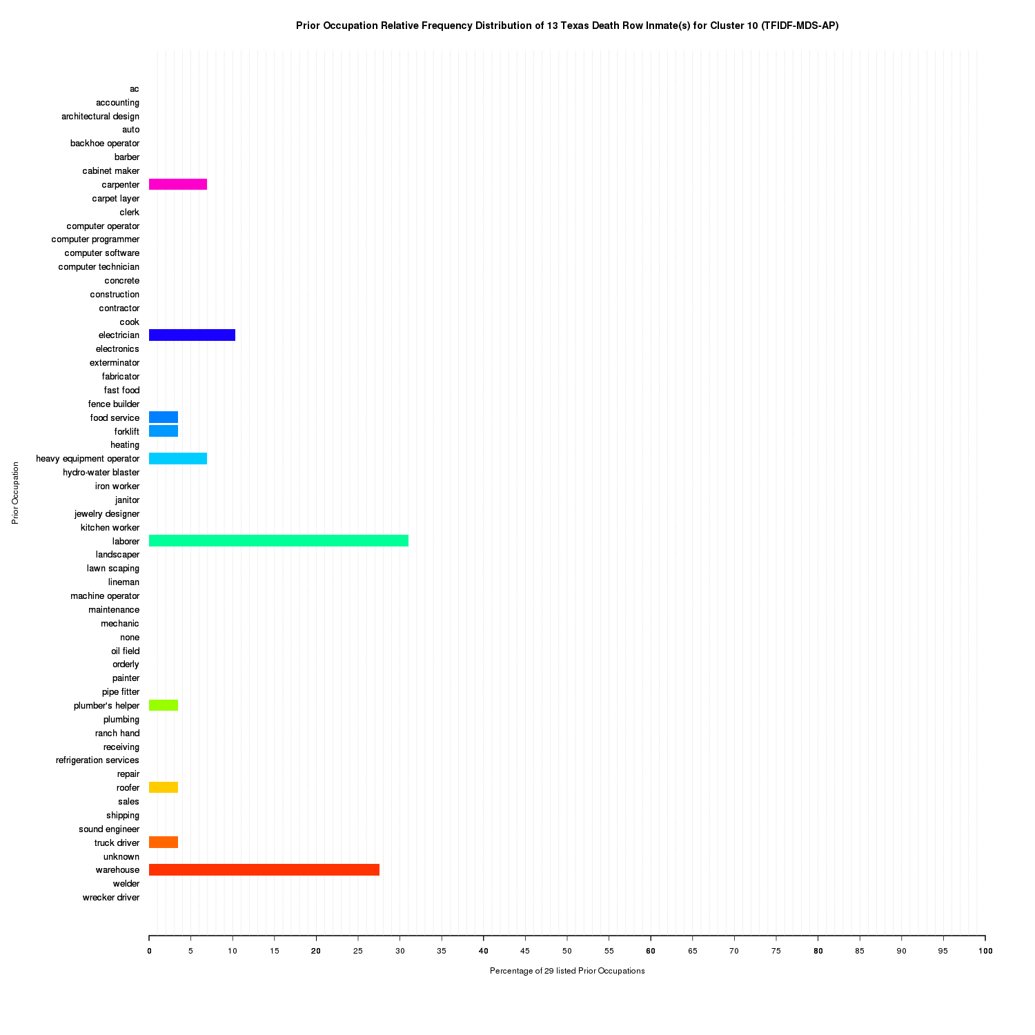
Prior Occupation Relative Frequency Distribution of 13 Texas Death Row Inmate(s) for Cluster 10 (TFIDF-MDS-AP)

For cluster 10, there is a large mixture of both laborer and warehouse.

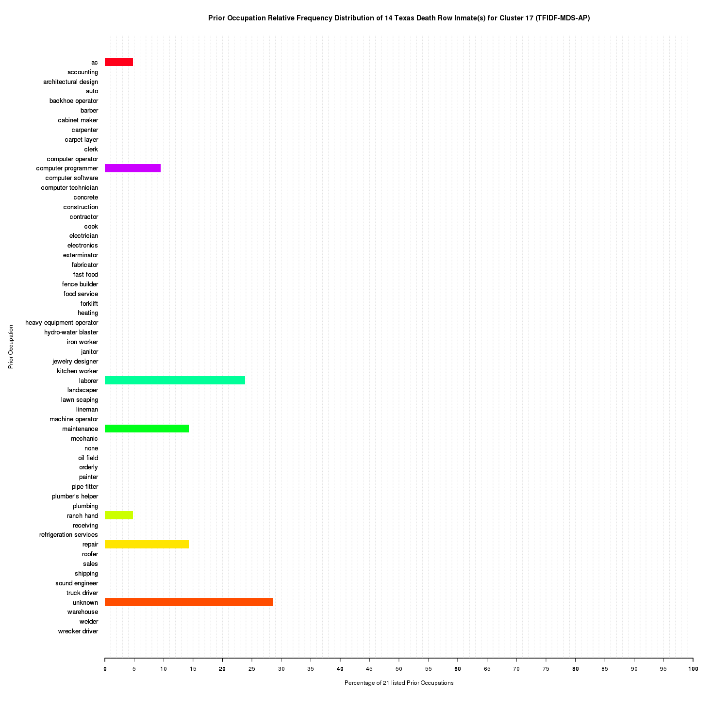
Prior Occupation Relative Frequency Distribution of 14 Texas Death Row Inmate(s) for Cluster 17 (TFIDF-MDS-AP)

Cluster 17 is more difficult to interpret and could have been likely clustered with cluster 5, however, it is the only cluster that accounts for the inmates that had unknown prior occupations. unknown did not collocate with any other prior occupation so it is surprising to find it clustered with other prior occupations. This is likely due to the MDS.

Automatic Cluster Labels

Using differential cluster labeling and more specifically pointwise mutual information (PMI), we can label each cluster according to its prior occupation with the highest association.

pc <- function(cn, b) {
  if (b == 1) {
    return(sum(input_cluster_labels == cn) / length(input_cluster_labels))
  } else {
    return(sum(input_cluster_labels != cn) / length(input_cluster_labels))
  }
}

pt <- function(ct, b) {
  if (b == 1) {
    in_d <- 0
    for (inmate_prior_occupations in inmates_prior_occupations) {
      count <- sum(ct == inmate_prior_occupations)
      if (count > 0) {
        in_d <- in_d + 1
      }
    }
    return(in_d / length(inmates_prior_occupations))
  } else {
    n_in_d <- 0
    for (inmate_prior_occupations in inmates_prior_occupations) {
      count <- sum(ct == inmate_prior_occupations)
      if (count == 0) {
        n_in_d <- n_in_d + 1
      }
    }
    return(n_in_d / length(inmates_prior_occupations))
  }
}

pct <- function(cn, ct, b) {
  if (all(b == c(0, 0))) {
    n_in_d <- 0
    inmate_indexes <- which(!input_cluster_labels %in% cn)
    for (inmate_index in inmate_indexes) {
      inmate_prior_occupations <- inmates_prior_occupations[[toString(inmate_index)]]
      count <- sum(ct == inmate_prior_occupations)
      if (count == 0) {
        n_in_d <- n_in_d + 1
      }
    }
    return(n_in_d / length(inmate_indexes))
  } else if (all(b == c(1, 1))) {
    in_d <- 0
    inmate_indexes <- which(input_cluster_labels %in% cn)
    for (inmate_index in inmate_indexes) {
      inmate_prior_occupations <- inmates_prior_occupations[[toString(inmate_index)]]
      count <- sum(ct == inmate_prior_occupations)
      if (count > 0) {
        in_d <- in_d + 1
      }
    }
    return(in_d / length(inmate_indexes))
  } else if (all(b == c(1, 0))) {
    n_in_d <- 0
    inmate_indexes <- which(input_cluster_labels %in% cn)
    for (inmate_index in inmate_indexes) {
      inmate_prior_occupations <- inmates_prior_occupations[[toString(inmate_index)]]
      count <- sum(ct == inmate_prior_occupations)
      if (count == 0) {
        n_in_d <- n_in_d + 1
      }
    }
    return(n_in_d / length(inmate_indexes))
  } else if (all(b == c(0, 1))) {
    in_d <- 0
    inmate_indexes <- which(!input_cluster_labels %in% cn)
    for (inmate_index in inmate_indexes) {
      inmate_prior_occupations <- inmates_prior_occupations[[toString(inmate_index)]]
      count <- sum(ct == inmate_prior_occupations)
      if (count > 0) {
        in_d <- in_d + 1
      }
    }
    return(in_d / length(inmate_indexes))
  }
}

pmi <- function(cn, ct) {
  pmi_score <- 0
  for (in_c in 0:1) {
    for (has_t in 0:1) {
      jpct_r <- pct(cn, ct, c(in_c, has_t))
      pc_r <- pc(cn, in_c)
      pt_r <- pt(ct, has_t)
      result <- jpct_r * log2(jpct_r / (pc_r * pt_r))
      if (is.nan(result)) {
        result <- 0
      }
      pmi_score <- pmi_score + result
    }
  }
  return(pmi_score)
}

output_cluster_labels <- list()
for(i in 1:length(inmate_clusters_str)) {
  cluster <- inmate_clusters_str[[toString(i)]]
  label <- ''
  max_pmi_score <- -1.0
  seen <- c()
  for (inmate in cluster) {
    for (prior_occupation in inmate) {
      if (sum(prior_occupation == seen) == 0) {
        pmi_score <- pmi(i, prior_occupation)
        if (pmi_score > max_pmi_score) {
          output_cluster_labels[[toString(i)]] <- prior_occupation
          max_pmi_score <- pmi_score
        }
        seen <- c(seen, prior_occupation)
      }
    }
  }
}

Cluster 1: none
Cluster 2: mechanic
Cluster 3: mechanic
Cluster 4: construction
Cluster 5: laborer
Cluster 6: cook
Cluster 7: welder
Cluster 8: welder
Cluster 9: ac
Cluster 10: warehouse
Cluster 11: construction
Cluster 12: clerk
Cluster 13: shipping
Cluster 14: clerk
Cluster 15: welder
Cluster 16: mechanic
Cluster 17: unknown

Condensing these even further:

none: cluster 1
mechanic: cluster 2, 3, 16
construction: cluster 4, 11
laborer: cluster 5
cook: cluster 6
welder: cluster 7, 8, 15
ac: cluster 9
warehouse: cluster 10
clerk: cluster 12, 14
shipping: cluster 13
unknown: cluster 17

This effectively condenses down the original 60 prior occupations down to the 11 most prominent in the sampled data. These 11 prior occupations could all be described as blue-collar occupations with the exception of clerk.

TF-IDF AP Clustering Only

Comparing the TF-IDF MDS AP clusters to TF-IDF AP clusters, using only the inmate_matrix_tfidf, the Affinity Propagation clustering algorithm generated 48 clusters using the original 60 dimensions versus the 17 clusters generated using the two dimensions found by MDS.

These 48 clusters are more granular with a clearer partitioning of inmates with unique prior occupations. 30 out of the 48 clusters contain only one inmate due to their unique combination of prior occupations. Cluster membership ranges from one to 71. Like with the MDS clusters, none is its own cluster. However, unlike the MDS clusters, all of the unknown prior occupations are clustered together alone.

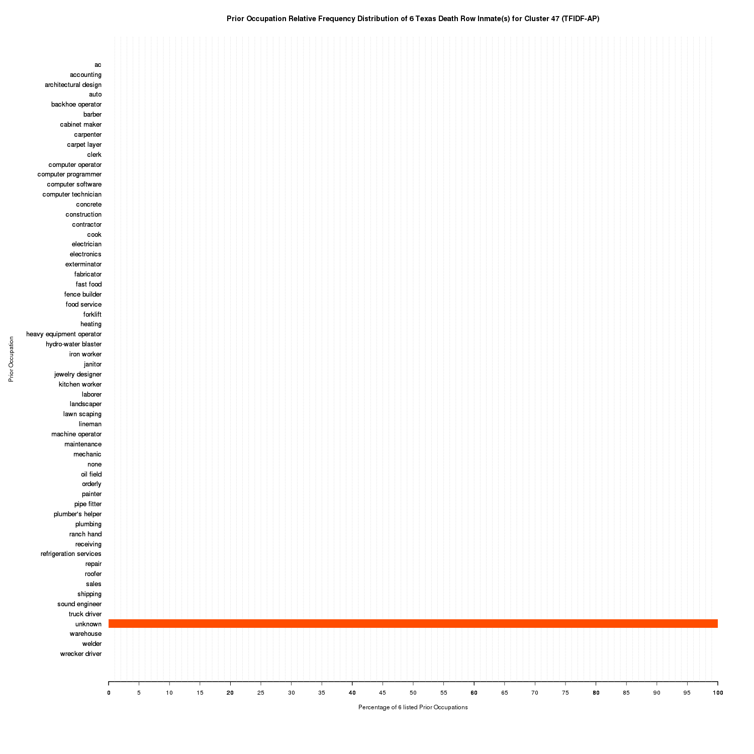
Prior Occupation Relative Frequency Distribution of 6 Texas Death Row Inmate(s) for Cluster 47 (TFIDF-AP)

Latent Semantic Indexing (LSI), Singular Value Decomposition (SVD)

We can take the TF-IDF normalized inmate-prior-occupation matrix and perform SVD on it.

LSI can be viewed as soft clustering by interpreting each dimension of the reduced space as a cluster and the value that a document has on that dimension as its fractional membership in that cluster.
Introduction to Information Retrieval

This will give us three matrices U, D, and V. U contains our inmate-concept vectors in the new orthogonal basis.

# -----------------------
# SVD
# -----------------------

inmate_matrix_tfidf_svd <- svd(inmate_matrix_tfidf)
k <- 38
inmate_k_basis_vectors = inmate_matrix_tfidf_svd$u[, 1:k]
k_singular_values_matrix = diag(inmate_matrix_tfidf_svd$d)[1:k, 1:k]
inmate_matrix_tfidf_svd_truncated <- inmate_k_basis_vectors %*% k_singular_values_matrix %*% t(inmate_matrix_tfidf_svd$v[, 1:k])

png(file='svd_explained_variance.png', width=1500, height=1500)
plot.new()
cumulativeVarianceExplained = cumsum(inmate_matrix_tfidf_svd$d^2 / sum(inmate_matrix_tfidf_svd$d^2)) * 100
plot(
  cumulativeVarianceExplained,
  type='o',
  ylim=c(0,100),
  xlab='Index',
  ylab='Percent of Variability Explained',
  main='Singular Value Decomposition'
)
axis(1, at=seq(1,length(inmate_matrix_tfidf_svd$d)))
abline(v=k)
abline(h=90.0)

bar_colors <- c()
for (i in 1:length(inmate_matrix_tfidf_svd$d)) {
  if (i == k) {
    bar_colors <- c(bar_colors, 'brown2')
  } else {
    bar_colors <- c(bar_colors, 'chartreuse3')
  }
}
png(
  file='svd_singular_values.png',
  width=1500,
  height=1500,
)
plot.new()
barplot(
  inmate_matrix_tfidf_svd$d,
  names.arg=1:length(inmate_matrix_tfidf_svd$d),
  col=bar_colors,
  ylim=c(0, max(inmate_matrix_tfidf_svd$d) + 1),
  border=NA,
  xlab='Index',
  ylab='Singular Value',
  main='Singular Value Decomposition'
)

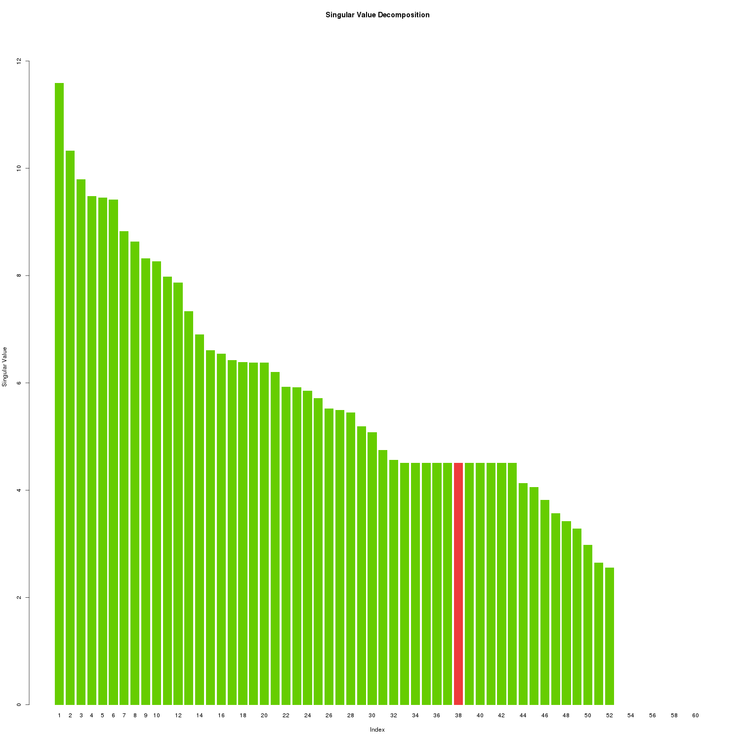
SVD Singular Values

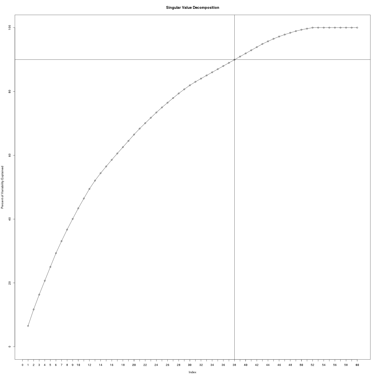
SVD Explained Variance

We’ll need to choose a K <= R (R being the rank) where R=60. At K=38, 90% of the variability of the original matrix is explained.

Now let us cluster and plot the prior occupation relative frequency distribution for each resulting cluster.

result <- cluster_matrix('TFIDF-SVD-AP', inmate_k_basis_vectors, inmates_prior_occupations)
inmate_clusters_flt <- result$flt
inmate_clusters_str <- result$str
inmate_clusters_colors <- result$colors
inmate_cluster_labels <- result$in_labels
inmate_clusters_labels <- result$out_labels

if (k == 2) {
  plot_clustering(
    'TFIDF-SVD-AP',
    inmate_k_basis_vectors,
    inmate_clusters_flt,
    inmate_clusters_colors,
    inmate_cluster_labels
  )
}
plot_clusters_occupation_distributions('TFIDF-SVD-AP', inmate_clusters_str, unique_prior_occupations)

After clustering, 40 clusters were found. Contrast this with the 48 found by TF-IDF alone which used 60 features instead the 38 used after applying SVD. Cluster membership ranges from one to 71.

Below are the cluster labels found by PMI:

Cluster 1: computer operator
Cluster 2: none
Cluster 3: kitchen worker
Cluster 4: computer programmer
Cluster 5: construction
Cluster 6: warehouse
Cluster 7: landscaper
Cluster 8: cabinet maker
Cluster 9: sales
Cluster 10: pipe fitter
Cluster 11: laborer
Cluster 12: barber
Cluster 13: machine operator
Cluster 14: truck driver
Cluster 15: oil field
Cluster 16: food service
Cluster 17: roofer
Cluster 18: fabricator
Cluster 19: cook
Cluster 20: computer technician
Cluster 21: janitor
Cluster 22: wrecker driver
Cluster 23: painter
Cluster 24: hydro-water blaster
Cluster 25: ranch hand
Cluster 26: heavy equipment operator
Cluster 27: iron worker
Cluster 28: shipping
Cluster 29: computer software
Cluster 30: clerk
Cluster 31: plumber's helper
Cluster 32: welder
Cluster 33: mechanic
Cluster 34: carpenter
Cluster 35: forklift
Cluster 36: heating
Cluster 37: unkown
Cluster 38: food service
Cluster 39: jewelry designer
Cluster 40: ac

Recap

We collected, parsed, and mined the prior occupations of current death row inmates. Interesting patterns discovered were the large portion of blue-collar occupations (most notably laborer) and more rare prior occupations such as computer operator and jewelry designer. An interesting hypothesis test would be the correlation between being on death row and having been a laborer. The SVD computation could be used for information retrieval allowing one to search for similar current inmates by some prior occupation query. Further analysis could include plotting the amount of each prior occupation seen per year.

Appendix

Full SVD AP Clustering

Computer operator Cluster 1
  Inmate 1 computer operator

None Cluster 2
  Inmate 3 none
  Inmate 4 none
  Inmate 8 none
  Inmate 13 none
  Inmate 18 none
  Inmate 41 none
  Inmate 42 none
  Inmate 44 none
  Inmate 50 none
  Inmate 61 none
  Inmate 63 none
  Inmate 65 none
  Inmate 66 none
  Inmate 68 none
  Inmate 177 none

Kitchen worker Cluster 3
  Inmate 10 c("kitchen worker", "construction")
  Inmate 48 kitchen worker

Computer programmer Cluster 4
  Inmate 11 computer programmer
  Inmate 156 c("computer programmer", "repair", "laborer")

Construction Cluster 5
  Inmate 7 c("construction", "plumbing")
  Inmate 15 construction
  Inmate 16 construction
  Inmate 17 construction
  Inmate 45 construction
  Inmate 47 construction
  Inmate 54 construction
  Inmate 116 c("construction", "laborer")

Warehouse Cluster 6
  Inmate 5 c("warehouse", "construction")
  Inmate 12 warehouse
  Inmate 22 c("warehouse", "laborer")
  Inmate 109 c("warehouse", "laborer")
  Inmate 112 c("warehouse", "electrician", "laborer")

Landscaper Cluster 7
  Inmate 25 c("landscaper", "cook")
  Inmate 69 c("landscaper", "laborer")

Cabinet maker Cluster 8
  Inmate 28 cabinet maker

Sales Cluster 9
  Inmate 29 sales
  Inmate 147 c("sound engineer", "laborer")

Pipe fitter Cluster 10
  Inmate 33 pipe fitter
  Inmate 60 c("truck driver", "backhoe operator", "welder", "pipe fitter")

Laborer Cluster 11
  Inmate 6 repair
  Inmate 21 laborer
  Inmate 23 laborer
  Inmate 26 laborer
  Inmate 30 laborer
  Inmate 32 laborer
  Inmate 34 laborer
  Inmate 35 laborer
  Inmate 36 laborer
  Inmate 38 laborer
  Inmate 40 laborer
  Inmate 43 laborer
  Inmate 46 laborer
  Inmate 51 laborer
  Inmate 70 laborer
  Inmate 71 laborer
  Inmate 74 laborer
  Inmate 77 c("electrician", "laborer")
  Inmate 78 laborer
  Inmate 79 laborer
  Inmate 80 laborer
  Inmate 82 laborer
  Inmate 85 laborer
  Inmate 86 laborer
  Inmate 87 laborer
  Inmate 89 c("maintenance", "laborer")
  Inmate 90 laborer
  Inmate 91 laborer
  Inmate 94 laborer
  Inmate 95 laborer
  Inmate 96 laborer
  Inmate 97 laborer
  Inmate 98 laborer
  Inmate 99 laborer
  Inmate 100 c("fast food", "laborer")
  Inmate 104 laborer
  Inmate 107 laborer
  Inmate 110 laborer
  Inmate 111 c("fast food", "laborer")
  Inmate 113 c("maintenance", "laborer")
  Inmate 119 c("maintenance", "laborer")
  Inmate 121 laborer
  Inmate 122 laborer
  Inmate 127 laborer
  Inmate 128 laborer
  Inmate 129 laborer
  Inmate 130 laborer
  Inmate 132 laborer
  Inmate 133 laborer
  Inmate 134 laborer
  Inmate 136 laborer
  Inmate 138 laborer
  Inmate 139 laborer
  Inmate 140 laborer
  Inmate 142 laborer
  Inmate 144 laborer
  Inmate 145 laborer
  Inmate 149 laborer
  Inmate 150 laborer
  Inmate 151 laborer
  Inmate 152 laborer
  Inmate 154 laborer
  Inmate 157 laborer
  Inmate 163 laborer
  Inmate 166 laborer
  Inmate 171 laborer
  Inmate 174 laborer
  Inmate 175 laborer
  Inmate 176 laborer
  Inmate 179 laborer
  Inmate 181 laborer

Barber Cluster 12
  Inmate 39 c("barber", "laborer")

Machine operator Cluster 13
  Inmate 53 machine operator

Truck driver Cluster 14
  Inmate 20 truck driver
  Inmate 56 truck driver
  Inmate 57 truck driver
  Inmate 62 c("truck driver", "warehouse")
  Inmate 88 c("truck driver", "laborer")

Oil field Cluster 15
  Inmate 58 c("welder", "oil field", "architectural design", "construction")

Food service Cluster 16
  Inmate 59 c("food service", "clerk")

Roofer Cluster 17
  Inmate 64 roofer
  Inmate 72 c("mechanic", "roofer", "concrete")

Fabricator Cluster 18
  Inmate 75 c("fabricator", "refrigeration services")

Cook Cluster 19
  Inmate 37 cook
  Inmate 67 c("construction", "cook")
  Inmate 81 c("cook", "laborer")
  Inmate 83 c("cook", "laborer")
  Inmate 118 c("cook", "construction", "welder", "laborer")
  Inmate 124 c("cook", "welder", "laborer")
  Inmate 137 c("cook", "mechanic", "laborer")

Computer technician Cluster 20
  Inmate 84 c("computer technician", "laborer")

Janitor Cluster 21
  Inmate 92 c("janitor", "laborer")

Wrecker driver Cluster 22
  Inmate 93 c("wrecker driver", "construction", "lineman", "laborer")

Painter Cluster 23
  Inmate 73 painter
  Inmate 101 c("painter", "laborer")
  Inmate 120 c("painter", "construction", "laborer")

Hydro-water blaster Cluster 24
  Inmate 103 c("hydro-water blaster", "laborer")

Ranch hand Cluster 25
  Inmate 105 c("repair", "ranch hand", "laborer")

Heavy equipment operator Cluster 26
  Inmate 14 c("mechanic", "warehouse", "heavy equipment operator")
  Inmate 114 c("heavy equipment operator", "laborer")
  Inmate 162 c("carpenter", "heavy equipment operator", "laborer")

Iron worker Cluster 27
  Inmate 115 c("iron worker", "construction", "carpet layer", "laborer")

Shipping Cluster 28
  Inmate 123 c("shipping", "receiving", "clerk", "mechanic", "laborer")

Computer software Cluster 29
  Inmate 126 c("computer software", "accounting", "laborer")

Clerk Cluster 30
  Inmate 2 clerk
  Inmate 27 clerk
  Inmate 117 c("clerk", "welder", "laborer")
  Inmate 131 c("clerk", "laborer")
  Inmate 153 c("clerk", "orderly", "laborer")

"Plumber's helper" Cluster 31
  Inmate 141 c("electrician", "plumber's helper", "laborer")

Welder Cluster 32
  Inmate 19 welder
  Inmate 31 c("welder", "lawn scaping", "laborer")
  Inmate 55 welder
  Inmate 76 c("welder", "fence builder")
  Inmate 135 c("welder", "contractor", "laborer")
  Inmate 143 c("welder", "laborer")

Mechanic Cluster 33
  Inmate 9 c("mechanic", "welder")
  Inmate 52 c("mechanic", "welder", "laborer")
  Inmate 146 c("mechanic", "laborer")
  Inmate 148 c("electrician", "mechanic", "laborer")
  Inmate 158 c("mechanic", "laborer")
  Inmate 161 c("auto", "mechanic", "laborer")
  Inmate 182 mechanic

Carpenter Cluster 34
  Inmate 106 c("warehouse", "carpenter", "laborer")
  Inmate 108 c("maintenance", "carpenter", "laborer")
  Inmate 125 c("welder", "carpenter", "laborer")
  Inmate 155 c("carpenter", "laborer")
  Inmate 164 c("carpenter", "laborer")

Forklift Cluster 35
  Inmate 24 c("forklift", "warehouse")
  Inmate 49 c("laborer", "forklift")
  Inmate 159 c("forklift", "laborer")

Heating Cluster 36
  Inmate 160 c("heating", "ac", "electronics", "exterminator", "laborer")

Unknown Cluster 37
  Inmate 165 unknown
  Inmate 167 unknown
  Inmate 168 unknown
  Inmate 169 unknown
  Inmate 172 unknown
  Inmate 173 unknown

Food service Cluster 38
  Inmate 170 c("warehouse", "food service", "laborer")

Jewelry designer Cluster 39
  Inmate 178 jewelry designer

Ac Cluster 40
  Inmate 102 c("ac", "repair", "electrician", "laborer")
  Inmate 180 ac

Full Source Code

# -----------------------
# (C) 2016 David lettier
# http://www.lettier.com/
# -----------------------

library(rvest)
library(wordcloud)
library(tm)
library(apcluster)

# -----------------------
# Scraping
# -----------------------

base_link <- 'https://www.tdcj.state.tx.us/death_row/'
main_link <- 'https://www.tdcj.state.tx.us/death_row/dr_offenders_on_dr.html'
csv_filename <- 'prior_occupations_dirty.csv'

if (!file.exists(csv_filename)) {
  page <- read_html(main_link)
  links <- html_attr(html_nodes(page, 'a'), 'href')
  links <- grep('^dr_info.*html$', links, value=TRUE)
  prior_occupations_dirty <- c()
  for (link in links) {
    texts <- read_html(paste(base_link, link, sep='')) %>% html_nodes('p') %>% html_text()
    if (length(grep('Prior Prison', texts[3])) >= 1) {
      prior_occupations_dirty <- c(prior_occupations_dirty, texts[2])
    } else {
      prior_occupations_dirty <- c(prior_occupations_dirty, texts[3])
    }
  }
  prior_occupations_dirty_df = as.data.frame(prior_occupations_dirty)
  write.csv(prior_occupations_dirty_df, file=csv_filename)
}

# -----------------------
# Cleaning
# -----------------------

csv_file <- read.csv(file=csv_filename)
prior_occupations_dirty <- as.vector(t(csv_file$prior_occupations_dirty))

prior_occupations_cleaned = c()
inmates_prior_occupations = list()
i <- 1
for (prior_occupation_dirty in prior_occupations_dirty) {
  prior_occupation <- gsub('Prior Occupation', '', prior_occupation_dirty)
  prior_occupation <- tolower(prior_occupation)
  prior_occupation <- gsub('^\\W+|^\\s+', ' ', prior_occupation)
  prior_occupation <- gsub('`', '', prior_occupation)
  prior_occupation <- gsub(':', ' ', prior_occupation)
  prior_occupation <- gsub('\\.', ' ', prior_occupation)
  prior_occupation <- gsub('\r', ' ', prior_occupation)
  prior_occupation <- gsub('\n', ' ', prior_occupation)
  prior_occupation <- gsub('\\s+', ' ', prior_occupation)
  if (length(grep('n/a', prior_occupation)) == 0) {
    prior_occupation <- gsub('/', ', ', prior_occupation)
  }
  prior_occupation <- gsub(' and ', ', ', prior_occupation)
  prior_occupation <- gsub('&', ', ', prior_occupation)
  prior_occupation <- gsub(';', ', ', prior_occupation)
  prior_occupation <- trimws(prior_occupation)
  prior_occupations <- strsplit(prior_occupation, ', ')
  prior_occupations <- lapply(prior_occupations, function (x) return(gsub('\\s+', ' ', x)))
  prior_occupations <- lapply(prior_occupations, function (x) return(trimws(x)))
  if (length(prior_occupations[[1]]) > 0) {
    prior_occupations_cleaned <- c(prior_occupations_cleaned, prior_occupations, recursive=T)
    inmates_prior_occupations[[toString(i)]] <- prior_occupations[[1]]
    i <- i + 1
  }
}
total_inmate_count = length(inmates_prior_occupations)

# -----------------------
# Duplication Removal
# -----------------------

prior_occupations_merged = c()
prior_occupations_merged_map = list()
for (prior_occupation_cleaned1 in prior_occupations_cleaned) {
  prior_occupation <- prior_occupation_cleaned1
  if (is.null(prior_occupations_merged_map[[prior_occupation]])) {
    if (nchar(prior_occupation) >= 4) {
      for (prior_occupation_cleaned2 in prior_occupations_cleaned) {
        if (nchar(prior_occupation_cleaned2) >= 4) {
          if (length(grep(prior_occupation_cleaned2, prior_occupation)) > 0) {
            if (nchar(prior_occupation) >= nchar(prior_occupation_cleaned2)) {
              prior_occupation <- prior_occupation_cleaned2
            }
          }
        }
      }
    }
    if (prior_occupation == 'n/a') {
      prior_occupation <- 'none'
    }
    if (length(grep('air condition', prior_occupation)) > 0) {
      prior_occupation <- 'ac'
    }
    if (length(grep('fork lift', prior_occupation)) > 0) {
      prior_occupation <- 'forklift'
    }
    if (length(grep('forklift', prior_occupation)) > 0) {
      prior_occupation <- 'forklift'
    }
    if (length(grep('clerical', prior_occupation)) > 0) {
      prior_occupation <- 'clerk'
    }
    if (length(grep('welding', prior_occupation)) > 0) {
      prior_occupation <- 'welder'
    }
    prior_occupations_merged_map[[prior_occupation_cleaned1]] <- prior_occupation
  } else {
    prior_occupation <- prior_occupations_merged_map[[prior_occupation]]
  }
  prior_occupations_merged <- c(prior_occupations_merged, prior_occupation)
}
total_prior_occupation_count = length(prior_occupations_merged)

i <- 1
for (inmate_prior_occupations in inmates_prior_occupations) {
  temp = c()
  for (prior_occupation in inmate_prior_occupations) {
    temp <- c(temp, prior_occupations_merged_map[[prior_occupation]])
  }
  inmates_prior_occupations[[toString(i)]] <- temp
  i <- i + 1
}
unique_prior_occupations = sort(unique(prior_occupations_merged))
unique_prior_occupations_length <- length(unique_prior_occupations)

# -----------------------
# Prior Occupation Relative Frequency Chart
# -----------------------

reverse_table <- function(t) { t[sort(names(t), decreasing=T)] }

prior_occupations_table <- reverse_table(table(prior_occupations_merged))
prior_occupations_table <- prior_occupations_table / sum(prior_occupations_table) * 100
png(file='prior_occupation_relative_freq_dist.png', width=1500, height=1500)
par(
  mai=c(2.0, 3.0, 1.0, 1.0)
)
barplot(
  prior_occupations_table,
  horiz=T,
  col=rainbow(length(prior_occupations_table)),
  cex.names=1.1,
  las=1,
  xlim=c(0, 100),
  axes=T,
  border=NA
)
axis(1, at=seq(0,100,5))
grid(nx=100, ny=NA)
barplot(
  prior_occupations_table,
  horiz=T,
  col=rainbow(length(prior_occupations_table)),
  cex.names=1.1,
  border=NA,
  las=1,
  xlim=c(0, 100),
  axes=T,
  add=T,
  xlab=paste('Percentage of', total_prior_occupation_count, 'listed Prior Occupations'),
  main=paste('Prior Occupation Relative Frequency Distribution of', total_inmate_count, 'Texas Death Row Inmates')
)
mtext('Prior Occupation', side=2, line=13)

# -----------------------
# Inmate x Prior Occupations
# -----------------------

inmate_matrix_count <- c()
for (row in 1:length(inmates_prior_occupations)) {
  inmate_prior_occupations <- inmates_prior_occupations[[toString(row)]]
  for (unique_prior_occupation in unique_prior_occupations) {
    inmate_matrix_count <- c(
      inmate_matrix_count,
      sum(unique_prior_occupation == inmate_prior_occupations)
    )
  }
}
inmate_matrix_count = matrix(
  inmate_matrix_count,
  nrow=total_inmate_count,
  ncol=unique_prior_occupations_length,
  byrow=T
)

# -----------------------
# TF-IDF
# -----------------------

inmate_matrix_tfidf <- matrix(
  c(
    1:(total_inmate_count * unique_prior_occupations_length)
  ) * 0,
  nrow=total_inmate_count,
  ncol=unique_prior_occupations_length,
  byrow=T
)
nrow_count <- nrow(inmate_matrix_count)
for (row in 1:nrow(inmate_matrix_count)) {
  for (col in 1:ncol(inmate_matrix_count)) {
    tf <- inmate_matrix_count[row,col]
    df <- length(which(inmate_matrix_count[,col] > 0))
    idf <- log(nrow_count / (df + 1))
    tfidf <- tf * idf
    inmate_matrix_tfidf[row,col] <- tfidf
  }
}

inmate_matrix_tfidf_l2_norm = c()
for (row in 1:nrow(inmate_matrix_tfidf)) {
  row_vector <- inmate_matrix_tfidf[row,]
  row_vector_norm <- row_vector/(sqrt(sum(row_vector^2)))
  inmate_matrix_tfidf_l2_norm = c(
    inmate_matrix_tfidf_l2_norm,
    row_vector_norm
  )
}
inmate_matrix_tfidf_l2_norm <- matrix(
  inmate_matrix_tfidf_l2_norm,
  nrow=total_inmate_count,
  ncol=unique_prior_occupations_length,
  byrow=T
)

# Uncomment to use the L2 norm version of TF-IDF.
# inmate_matrix_tfidf <- inmate_matrix_tfidf_l2_norm

# -----------------------
# MDS
# -----------------------

plot_scale <- 1.0

scatter_plot_matrix <- function(prefix, input_matrix) {
  png(file=paste(tolower(prefix), 'scatter_plot.png', sep='_'), width=1500, height=1500)
  plot.new()
  input_matrix[,1]
  input_matrix[,2]
  textplot(
    input_matrix[, 1],
    input_matrix[, 2],
    seq(1:length(input_matrix[,1])),
    xlim=c(
      min(input_matrix[, 1]) * plot_scale,
      max(input_matrix[, 1]) * plot_scale
    ),
    ylim=c(
      min(input_matrix[, 2]) * plot_scale,
      max(input_matrix[, 2]) * plot_scale
    ),
    main=paste('Inmate Prior Occupations 2D Visualization', paste0('(', prefix, ')'))
  )
}

dist_matrix <- dist(inmate_matrix_count, method='euclidean')
inmate_matrix_count_mds <- cmdscale(dist_matrix)
scatter_plot_matrix('COUNT-MDS', inmate_matrix_count_mds)

dist_matrix <- dist(inmate_matrix_tfidf, method='euclidean')
inmate_matrix_tfidf_mds <- cmdscale(dist_matrix)
scatter_plot_matrix('TFIDF-MDS', inmate_matrix_tfidf_mds)

# -----------------------
# AP CLUSTERING
# -----------------------

cluster_matrix <- function(prefix, input_matrix, inmates_prior_occupations) {
  apresult <- apcluster(negDistMat(r=2), input_matrix)
  input_cluster_labels = labels(apresult, type='enum')

  inmate_clusters_flt <- list()
  inmate_clusters_str <- list()

  i <- 1
  for (input_cluster_label in input_cluster_labels) {
    input_cluster_label <- toString(input_cluster_label)

    if (is.null(inmate_clusters_flt[[input_cluster_label]])) {
      inmate_clusters_flt[[input_cluster_label]] <- c()
      inmate_clusters_str[[input_cluster_label]] <- list()
    }

    inmate_clusters_flt[[input_cluster_label]] <- c(
      inmate_clusters_flt[[input_cluster_label]],
      input_matrix[i,]
    )

    i_str <- toString(i)
    temp = list()
    temp[[i_str]] <- inmates_prior_occupations[[i_str]]
    inmate_clusters_str[[input_cluster_label]] <- append(
      inmate_clusters_str[[input_cluster_label]],
      temp
    )

    i <- i + 1
  }

  for (cluster_i in 1:length(inmate_clusters_flt)) {
    cluster_i_str <- toString(cluster_i)
    cluster <- matrix(inmate_clusters_flt[[cluster_i_str]], ncol=2, byrow=T)
    inmate_clusters_flt[[cluster_i_str]] <- cluster
  }

  inmate_clusters_colors = rainbow(length(inmate_clusters_flt), v=0.8, s=0.5)

  pc <- function(cn, b) {
    if (b == 1) {
      return(sum(input_cluster_labels == cn) / length(input_cluster_labels))
    } else {
      return(sum(input_cluster_labels != cn) / length(input_cluster_labels))
    }
  }

  pt <- function(ct, b) {
    if (b == 1) {
      in_d <- 0
      for (inmate_prior_occupations in inmates_prior_occupations) {
        count <- sum(ct == inmate_prior_occupations)
        if (count > 0) {
          in_d <- in_d + 1
        }
      }
      return(in_d / length(inmates_prior_occupations))
    } else {
      n_in_d <- 0
      for (inmate_prior_occupations in inmates_prior_occupations) {
        count <- sum(ct == inmate_prior_occupations)
        if (count == 0) {
          n_in_d <- n_in_d + 1
        }
      }
      return(n_in_d / length(inmates_prior_occupations))
    }
  }

  pct <- function(cn, ct, b) {
    if (all(b == c(0, 0))) {
      n_in_d <- 0
      inmate_indexes <- which(!input_cluster_labels %in% cn)
      for (inmate_index in inmate_indexes) {
        inmate_prior_occupations <- inmates_prior_occupations[[toString(inmate_index)]]
        count <- sum(ct == inmate_prior_occupations)
        if (count == 0) {
          n_in_d <- n_in_d + 1
        }
      }
      return(n_in_d / length(inmate_indexes))
    } else if (all(b == c(1, 1))) {
      in_d <- 0
      inmate_indexes <- which(input_cluster_labels %in% cn)
      for (inmate_index in inmate_indexes) {
        inmate_prior_occupations <- inmates_prior_occupations[[toString(inmate_index)]]
        count <- sum(ct == inmate_prior_occupations)
        if (count > 0) {
          in_d <- in_d + 1
        }
      }
      return(in_d / length(inmate_indexes))
    } else if (all(b == c(1, 0))) {
      n_in_d <- 0
      inmate_indexes <- which(input_cluster_labels %in% cn)
      for (inmate_index in inmate_indexes) {
        inmate_prior_occupations <- inmates_prior_occupations[[toString(inmate_index)]]
        count <- sum(ct == inmate_prior_occupations)
        if (count == 0) {
          n_in_d <- n_in_d + 1
        }
      }
      return(n_in_d / length(inmate_indexes))
    } else if (all(b == c(0, 1))) {
      in_d <- 0
      inmate_indexes <- which(!input_cluster_labels %in% cn)
      for (inmate_index in inmate_indexes) {
        inmate_prior_occupations <- inmates_prior_occupations[[toString(inmate_index)]]
        count <- sum(ct == inmate_prior_occupations)
        if (count > 0) {
          in_d <- in_d + 1
        }
      }
      return(in_d / length(inmate_indexes))
    }
  }

  pmi <- function(cn, ct) {
    pmi_score <- 0
    for (in_c in 0:1) {
      for (has_t in 0:1) {
        jpct_r <- pct(cn, ct, c(in_c, has_t))
        pc_r <- pc(cn, in_c)
        pt_r <- pt(ct, has_t)
        result <- jpct_r * log2(jpct_r / (pc_r * pt_r))
        if (is.nan(result)) {
          result <- 0
        }
        pmi_score <- pmi_score + result
      }
    }
    return(pmi_score)
  }

  output_cluster_labels <- list()
  for(i in 1:length(inmate_clusters_str)) {
    cluster <- inmate_clusters_str[[toString(i)]]
    label <- ''
    max_pmi_score <- -1.0
    seen <- c()
    for (inmate in cluster) {
      for (prior_occupation in inmate) {
        if (sum(prior_occupation == seen) == 0) {
          pmi_score <- pmi(i, prior_occupation)
          if (pmi_score > max_pmi_score) {
            output_cluster_labels[[toString(i)]] <- prior_occupation
            max_pmi_score <- pmi_score
          }
          seen <- c(seen, prior_occupation)
        }
      }
    }
  }

  write(
    sapply(
      sort(as.integer(names(inmate_clusters_str))),
      function(x) paste(
        paste0(
          toupper(substring(output_cluster_labels[[toString(x)]], 1, 1)),
          substring(
            output_cluster_labels[[toString(x)]],
            2,
            nchar(output_cluster_labels[[toString(x)]])
          )
        ),
        'Cluster',
        toString(x),
        '\n ',
        paste('Inmate', names(inmate_clusters_str[[toString(x)]]), inmate_clusters_str[[toString(x)]], collapse='\n  ')
      )),
    paste(tolower(prefix), 'inmate_clusters.txt', sep='_')
  )

  return(
    list(
      flt=inmate_clusters_flt,
      str=inmate_clusters_str,
      colors=inmate_clusters_colors,
      in_labels=input_cluster_labels,
      out_labels=output_cluster_labels
    )
  )
}

plot_clustering <- function(prefix, input_matrix, inmate_cluster_flt, inmate_clusters_colors, inmate_cluster_labels) {
  png(file=paste(tolower(prefix), 'inmate_clusters.png', sep='_'), width=1500, height=1500)
  plot.new()
  plot(
    input_matrix[,1],
    input_matrix[,2],
    main=paste('Death Row Inmate Clustering by Prior Occupations', paste0('(', prefix, ')'))
  )
  for (cluster_i in 1:length(inmate_clusters_flt)) {
    cluster_i_str <- toString(cluster_i)
    points(
      inmate_clusters_flt[[cluster_i_str]],
      col=inmate_clusters_colors[cluster_i],
      bg=inmate_clusters_colors[cluster_i],
      pch=19,
      cex=5,
      lwd=2
    )
  }
  text(
    input_matrix[, 1],
    input_matrix[, 2],
    inmate_cluster_labels,
    xlim=c(
      min(input_matrix[, 1]) * plot_scale,
      max(input_matrix[, 1]) * plot_scale
    ),
    ylim=c(
      min(input_matrix[, 2]) * plot_scale,
      max(input_matrix[, 2]) * plot_scale
    ),
  )
  legend(
    'topleft',
    legend=lapply(c(1:length(inmate_clusters_colors)), function (x) return(toString(x))),
    fill=inmate_clusters_colors,
    cex=1.3,
    pt.cex=1
  )
}

plot_clusters_occupation_distributions <- function(prefix, inmate_clusters_str, unique_prior_occupations) {
  for (i in 1:length(inmate_clusters_str)) {
    cluster <- inmate_clusters_str[[toString(i)]]
    cluster_prior_occupations <- c()
    for (inmate_prior_occupations in cluster) {
      cluster_prior_occupations <- c(cluster_prior_occupations, inmate_prior_occupations)
    }

    prior_occupations_table <- reverse_table(table(factor(cluster_prior_occupations, levels=unique_prior_occupations)))
    prior_occupations_table <- prior_occupations_table / sum(prior_occupations_table) * 100

    png(file=paste(tolower(prefix), toString(i), 'prior_occupation_distribution.png', sep='_'), width=1500, height=1500)
    plot.new()
    par(
      mai=c(2.0, 3.0, 1.0, 1.0)
    )
    barplot(
      prior_occupations_table,
      horiz=T,
      col=rainbow(length(prior_occupations_table)),
      cex.names=1.1,
      las=1,
      xlim=c(0, 100),
      axes=T,
      border=NA
    )
    axis(1, at=seq(0,100,5))
    grid(nx=100, ny=NA)
    barplot(
      prior_occupations_table,
      horiz=T,
      col=rainbow(length(prior_occupations_table)),
      cex.names=1.1,
      las=1,
      xlim=c(0, 100),
      axes=T,
      add=T,
      ylab='',
      xlab=paste('Percentage of', length(cluster_prior_occupations), 'listed Prior Occupations'),
      main=paste(
        'Prior Occupation Relative Frequency Distribution of',
        length(cluster),
        'Texas Death Row Inmate(s) for Cluster',
        toString(i),
        paste0(
          '(',
          prefix,
          ')'
        )
      ),
      border=NA
    )
    mtext('Prior Occupation', side=2, line=13)
    dev.off()
  }
}

result <- cluster_matrix('COUNT-AP', inmate_matrix_count, inmates_prior_occupations)
inmate_clusters_flt <- result$flt
inmate_clusters_str <- result$str
inmate_clusters_colors <- result$colors

plot_clusters_occupation_distributions('COUNT-AP', inmate_clusters_str, unique_prior_occupations)

result <- cluster_matrix('TFIDF-AP', inmate_matrix_tfidf, inmates_prior_occupations)
inmate_clusters_flt <- result$flt
inmate_clusters_str <- result$str
inmate_clusters_colors <- result$colors

plot_clusters_occupation_distributions('TFIDF-AP', inmate_clusters_str, unique_prior_occupations)

result <- cluster_matrix('COUNT-MDS-AP', inmate_matrix_count_mds, inmates_prior_occupations)
inmate_clusters_flt <- result$flt
inmate_clusters_str <- result$str
inmate_clusters_colors <- result$colors
inmate_cluster_labels <- result$in_labels
inmate_clusters_labels <- result$out_labels

plot_clustering('COUNT-MDS-AP', inmate_matrix_count_mds, inmate_clusters_flt, inmate_clusters_colors, inmate_cluster_labels)
plot_clusters_occupation_distributions('COUNT-MDS-AP', inmate_clusters_str, unique_prior_occupations)

result <- cluster_matrix('TFIDF-MDS-AP', inmate_matrix_tfidf_mds, inmates_prior_occupations)
inmate_clusters_flt <- result$flt
inmate_clusters_str <- result$str
inmate_clusters_colors <- result$colors
inmate_cluster_labels <- result$in_labels
inmate_clusters_labels <- result$out_labels

plot_clustering('TFIDF-MDS-AP', inmate_matrix_tfidf_mds, inmate_clusters_flt, inmate_clusters_colors, inmate_cluster_labels)
plot_clusters_occupation_distributions('TFIDF-MDS-AP', inmate_clusters_str, unique_prior_occupations)

# -----------------------
# SVD
# -----------------------

inmate_matrix_tfidf_svd <- svd(inmate_matrix_tfidf)
k <- 38
inmate_k_basis_vectors = inmate_matrix_tfidf_svd$u[, 1:k]
k_singular_values_matrix = diag(inmate_matrix_tfidf_svd$d)[1:k, 1:k]
inmate_matrix_tfidf_svd_truncated <- inmate_k_basis_vectors %*% k_singular_values_matrix %*% t(inmate_matrix_tfidf_svd$v[, 1:k])

png(file='svd_explained_variance.png', width=1500, height=1500)
plot.new()
cumulativeVarianceExplained = cumsum(inmate_matrix_tfidf_svd$d^2 / sum(inmate_matrix_tfidf_svd$d^2)) * 100
plot(
  cumulativeVarianceExplained,
  type='o',
  ylim=c(0,100),
  xlab='Index',
  ylab='Percent of Variability Explained',
  main='Singular Value Decomposition'
)
axis(1, at=seq(1,length(inmate_matrix_tfidf_svd$d)))
abline(v=k)
abline(h=90.0)

bar_colors <- c()
for (i in 1:length(inmate_matrix_tfidf_svd$d)) {
  if (i == k) {
    bar_colors <- c(bar_colors, 'brown2')
  } else {
    bar_colors <- c(bar_colors, 'chartreuse3')
  }
}
png(
  file='svd_singular_values.png',
  width=1500,
  height=1500,
)
plot.new()
barplot(
  inmate_matrix_tfidf_svd$d,
  names.arg=1:length(inmate_matrix_tfidf_svd$d),
  col=bar_colors,
  ylim=c(0, max(inmate_matrix_tfidf_svd$d) + 1),
  border=NA,
  xlab='Index',
  ylab='Singular Value',
  main='Singular Value Decomposition'
)

result <- cluster_matrix('TFIDF-SVD-AP', inmate_k_basis_vectors, inmates_prior_occupations)
inmate_clusters_flt <- result$flt
inmate_clusters_str <- result$str
inmate_clusters_colors <- result$colors
inmate_cluster_labels <- result$in_labels
inmate_clusters_labels <- result$out_labels

if (k == 2) {
  plot_clustering(
    'TFIDF-SVD-AP',
    inmate_k_basis_vectors,
    inmate_clusters_flt,
    inmate_clusters_colors,
    inmate_cluster_labels
  )
}
plot_clusters_occupation_distributions('TFIDF-SVD-AP', inmate_clusters_str, unique_prior_occupations)

Text Mining in R: Death Row Prior Occupations |