Birthday Condolences, Greeting Card Classifier by David Lettier

It is late and your cart of greeting cards just fell over mixing birthday and sympathy cards all over the floor. Unfortunately, you cannot go home until you restock the card shelves. Luckily you have OCR on your phone and a knack for machine learning. Let’s build a classifier using scikit-learn’s implementation of logistic regression.

Sample Data

Our sample data consists of four files:

positive.train.dat
negative.train.dat
positive.test.dat
negative.test.dat.

Below is the specific makeup:

Training:

  Positive:  84
  Negative: 100
  -------------
     Total: 184

Test:

  Positive: 100
  Negative:  50
  -------------
     Total: 150

The training examples we will use for parameter optimization and cross validation. Once we have built our predictive model, we’ll check its performance using our test set of examples the model never saw during training and validation.

The positive examples are birthday card greetings found on various websites around the web. Here is a small sample:

They say that with age comes wisdom. You must be one of the wisest.
To the nation’s best kept secret; Your true age.
What goes up but never comes down? Your age.
It’s your birthday. Now you have more grown up. Every year you’re becoming more perfect.
Wishing happy birthday to the best person I have ever met in this world.
Thank you for all the memories we have. Without you the world would have been colorless to me.

For the negative samples, we’ll use condolences which you would find in sympathy cards. Here is a small sample:

You and your family are in my heart and mind. My condolences on the passing of your father.
It’s terrible to hear about your loss and I express my sincere sympathy to you and your family
I am deeply saddened by the loss that you and your family have encountered. My condolences.
My deepest sympathies go out to you and your family. May God give you the peace that you seek.
May my condolences bring you comfort and may my prayers ease the pain of this loss.
I offer you my thoughts, prayers and well-wishes during this dark time in your life.

Our classes will be 1 for positive birthday greeting and 0 for negative not birthday greeting (sympathy).

Dependencies

We will need matplotlib for charting and sklearn for corpus processing, hyperparamter search, model building, and metrics calculations.

import operator
import matplotlib.pyplot as pyplot
from numpy.random import uniform
from sklearn.pipeline import Pipeline
from sklearn.feature_extraction.text import CountVectorizer
from sklearn.feature_extraction.text import TfidfVectorizer
from sklearn.grid_search import RandomizedSearchCV
from sklearn.linear_model import LogisticRegression
from sklearn.cross_validation import cross_val_score
from sklearn.metrics import log_loss
from sklearn.metrics import roc_auc_score
from sklearn.metrics import roc_curve

Loading the Data

Each sample occupies a single newline in each file. For each type (positive or negative) we’ll generate the class labels for each sample.

def load(file_name):
  with open(file_name) as f:
    lines = f.readlines()

  return [x.strip().lower() for x in lines]

positive_samples_train = load('positive.train.dat')
negative_samples_train = load('negative.train.dat')
samples_train = positive_samples_train + negative_samples_train
labels_train = [1 for x in positive_samples_train] + \
  [0 for x in negative_samples_train]

positive_samples_test = load('positive.test.dat')
negative_samples_test = load('negative.test.dat')
samples_test = positive_samples_test + negative_samples_test
labels_test = [1 for x in positive_samples_test] + \
  [0 for x in negative_samples_test]

Word frequencies per class

To get a sense of the feature landscape let’s calculate the top word frequencies found for both positive, negative, train and test.

def vocab_count(samples, typee):
  vocab_counter = CountVectorizer(
    stop_words='english',
    ngram_range=(1, 2),
    max_df=1.0,
    min_df=0.0
  )
  dtm = vocab_counter.fit_transform(samples)
  vocab_indexes = vocab_counter.get_feature_names()
  vocab_totals = {}
  for row in dtm:
    for j, count in enumerate(row.A[0]):
      word = vocab_indexes[j]
      vocab_totals[word] = vocab_totals.get(word, 0)
      vocab_totals[word] += count

  print(
    'Most frequent %s corpus features: %s' % (
      typee,
      sorted(
        vocab_totals.items(),
        key=operator.itemgetter(1),
        reverse=True
      )[:10]
    )
  )

vocab_count(positive_samples_train, 'positive training')
vocab_count(negative_samples_train, 'negative training')
vocab_count(positive_samples_test, 'positive test')
vocab_count(negative_samples_test, 'negative test')

Most frequent positive training corpus features:
  [
    ('birthday', 32),
    ('age', 17),
    ('happy', 15),
    ('old', 14),
    ('candles', 12),
    ('happy birthday', 11),
    ('people', 11),
    ('year', 10),
    ('like', 9),
    ('cake', 9)
  ]

Most frequent negative training corpus features:
  [
    ('condolences', 48),
    ('loss', 23),
    ('family', 22),
    ('peace', 21),
    ('soul', 20),
    ('god', 19),
    ('rest', 16),
    ('time', 16),
    ('comfort', 13),
    ('prayers', 13)
  ]

Most frequent positive test corpus features:
  [
    ('birthday', 101),
    ('happy', 87),
    ('happy birthday', 84),
    ('friend', 31),
    ('day', 24),
    ('best', 24),
    ('special', 22),
    ('life', 21),
    ('world', 21),
    ('love', 20)
  ]

Most frequent negative test corpus features:
  [
    ('condolences', 26),
    ('family', 19),
    ('insert', 17),
    ('deceased', 17),
    ('bereaved', 17),
    ('peace', 16),
    ('god', 14),
    ('soul', 14),
    ('deceased bereaved', 13),
    ('relationship', 13)
  ]

Even though it is early in the process, it is safe to say that birthday and condolences contain a lot of information about a greeting card’s class. The features birthday and condolences are not English stop-words nor are they stop-words for our particular corpus. Corpus specific stop-words are words found frequently in most/all classes providing little discrimination and a lot of overlap.

The Pipeline

For convenience we’ll setup a pipeline that will take our raw text, pre-process it, and then pass it to our logistic regression model.

pipeline = Pipeline(
  steps=[
    ('tfidf', TfidfVectorizer(ngram_range=(1, 2), stop_words='english')),
    ('logistic', LogisticRegression())
  ]
)

TF-IDF Weighting

Not all words found in the corpus are equally important. For each sample, we will weight each of its words by the ratio of how many times they appear in the sentence versus how many times they appear in all of the sentences using TF-IDF.

Logistic Regression

Our binary classifier of choice will be logistic regression. In some ways it is similar to linear regression but uses a different hypothesis function h(x) = 1 / (1 + e^(-Z)) where Z = θ^(T) * x. As an added bonus, the output of h is the positive class probability versus just a binary prediction of one or zero.

Randomized Search Cross Validation

Both the TF-IDF and logistic regression algorithms have hyperparameters that need to be defined up front. We could spend all day tweaking these and then cross validating but instead we’ll use scikit-learn’s RandomizedSearchCV. We’ll iterate 100 times doing 10-fold cross validation each time in order to find four hyperparamters: TF-IDF min-df (document frequency), TF-IDF max-df, logistic regression C (the inverse of the regularization strength), and the logistic regression regularization type or penalty. Our goal during our search is to minimize the logarithmic loss.

n = 100
k = 10
search = RandomizedSearchCV(
  pipeline,
  param_distributions={
    'tfidf__min_df': uniform(0.0, 0.2, n),
    'tfidf__max_df': uniform(0.8, 1.0, n),
    'logistic__C': uniform(0.0, 1.0, n),
    'logistic__penalty': ['l1', 'l2']
  },
  n_jobs=8,
  cv=k,
  scoring='log_loss',
  n_iter=n
)

The Best Hyperparameters

After performing the randomized search we arrive at:

Best hyperparams: {
  'tfidf__max_df': 0.84163294453018755,
  'tfidf__min_df': 0.053779330737934818,
  'logistic__penalty': 'l1',
  'logistic__C': 0.94865926441506498
}

The defaults are:

{
  'tfidf__max_df': 1.0,
  'tfidf__min_df': 1,
  'logistic__penalty': 'l2',
  'logistic__C': 1.0
}

TF-IDF vocabulary

Using the best hyperparameters found, let us take a look at the vocabulary or features actually used in the pipeline.

print(
  'TF-IDF Vocabulary: %s' % (
    [key for key, _ in tfidf.vocabulary_.items()],
  )
)

TF-IDF Vocabulary: [
 'god',
 'happy birthday',
 'know',
 'old',
 'prayers',
 'people',
 'words',
 'soul',
 'family',
 'age',
 'mother',
 'love',
 'comfort',
 'peace',
 'rest',
 'time',
 'candles',
 'happy',
 'like',
 'loss',
 'birthday',
 'great',
 'condolences'
]

Most of them are the same words listed above in the corpus word frequencies.

Log Loss Cross Validation Score

Using our best found model, we can now perform 10-fold cross validation using the log loss scoring function. Imagine splitting up the training samples into 10 chunks. You find the best weights for the model/function using 9 out of the 10 chunks. You then test the trained model on the 10^th chunk evaluating the log loss metric. Now do this 10 times until each chunk was used as the test chunk.

print(
  '%s-fold mean Log Loss CV score: %s' % (
    k,
    abs(  # scikit-learn outputs a negative score but log loss is non-negative
      cross_val_score(
        pipeline,
        samples_train,
        labels_train,
        scoring='log_loss',
        cv=k,
        n_jobs=8
      ).mean()
    ),
  )
)

10-fold mean Log Loss CV score: 0.28916885941

Test Metrics

Our model is now trained, validated, and ready for testing on some unseen data.

pipeline.fit(samples_train, labels_train)
classes = pipeline.classes_.tolist()

print('Classes: %s' % (classes,))

true = labels_test
pred_prob = pipeline.predict_proba(samples_test)
pred_prob_pos = [x[classes.index(1)] for x in pred_prob]

print(
  'Test Log Loss: %s' % (
    log_loss(
      true,
      pred_prob
    )
  )
)

print(
  'Test ROC AUC: %s' % (
    roc_auc_score(
      true,
      pred_prob_pos
    )
  )
)

Log Loss

The log loss score is very high when the classifier gives a very low class probability for a sample that is actually the class.

Test Log Loss: 0.164580415601

For example:

In [90]: true = [1] * 5 + [0] * 5 # First five are yes and last 5 are no.

# First five give 100% probability to it being a yes and 0% probability to it being a no.
# Last  five give 100% probability to it being a  no and 0% probability to it being a yes.
In [91]: pred = [[0.0, 1.0] for i in range(5)] + [[1.0, 0.0] for i in range(5)]
#                 no,  yes                         no,  yes

In [92]: log_loss(true, pred)
Out[92]: 9.9920072216264128e-16 # It predicted each one completely right.
#                          ^ very small.

In [93]: pred = pred[::-1] # Reverse it so it gets each one completely wrong.

In [94]: pred
Out[94]:
[[1.0, 0.0],
 [1.0, 0.0],
 [1.0, 0.0],
 [1.0, 0.0],
 [1.0, 0.0],
 [0.0, 1.0],
 [0.0, 1.0],
 [0.0, 1.0],
 [0.0, 1.0],
 [0.0, 1.0]]

In [95]: log_loss(true, pred)
Out[95]: 34.538776394910677

ROC AUC (Area under the Curve)

The ROC AUC is the area under the receiver operating characteristic curve (ROC). An area of one is a perfect score.

Test ROC AUC: 0.9976

To hammer home the last post, let’s chart the ROC curve by varying the class probability thresholds.

fpr, tpr, thresholds = roc_curve(true, pred_prob_pos, pos_label=1)
pyplot.style.use('ggplot')
pyplot.plot([0.0] + fpr.tolist(), [0.0] + fpr.tolist(), '--')
pyplot.plot([0.0] + fpr.tolist(), [0.0] + tpr.tolist())
pyplot.title(
  'ROC Curve',
  y=1.08
)
pyplot.suptitle(
  'Logistic Regression Classifier '
  'of Birthday Wishes vs Condolences',
  y=0.95
)
pyplot.xlabel('False Positive Rate')
pyplot.ylabel('True Positive Rate')
pyplot.xlim([-0.05, 1.05])
pyplot.ylim([-0.05, 1.05])
pyplot.savefig('roc_curve.png')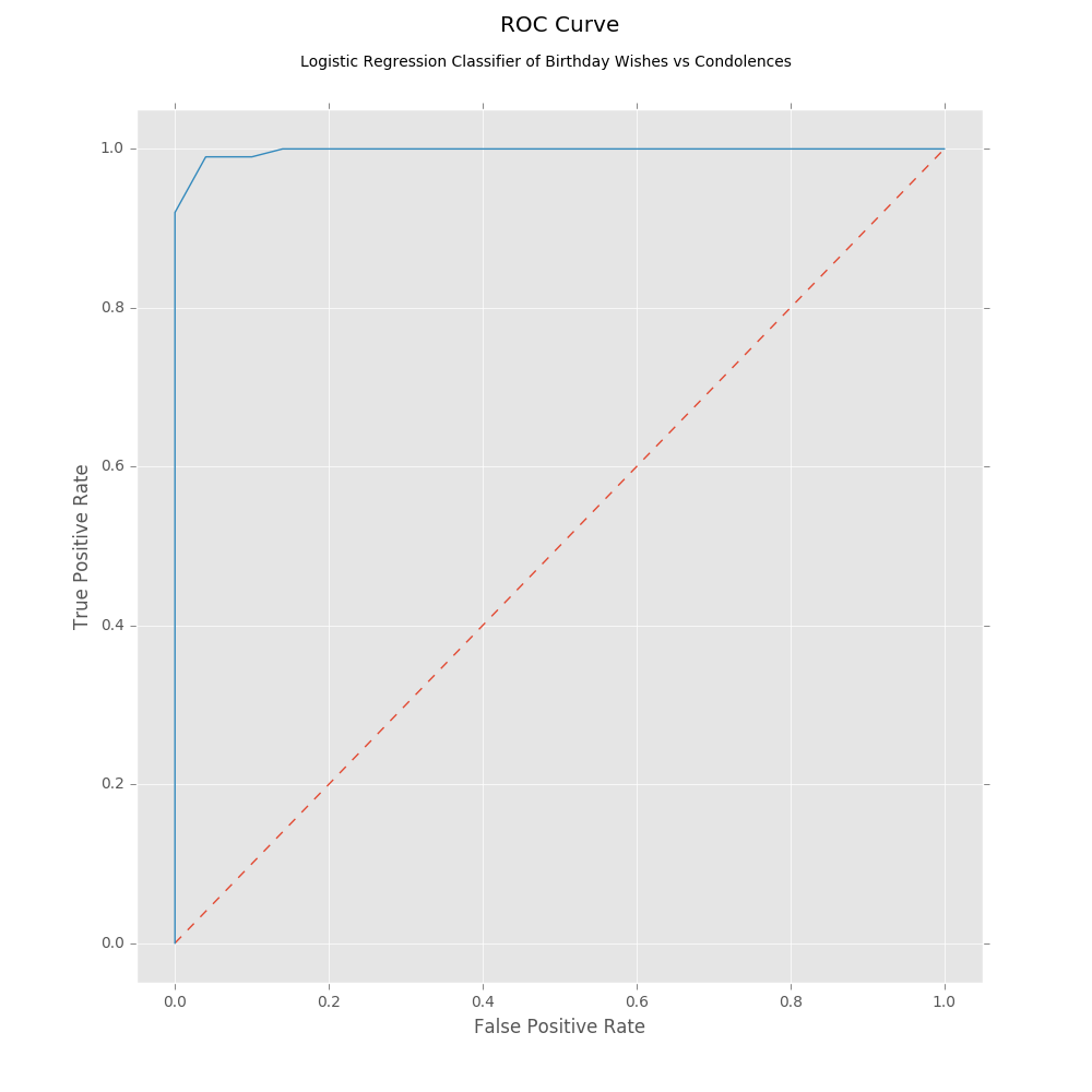

ROC Curve

Recap

We explored our sample data set and held out some examples for testing. After building our pre-processing and model pipeline, we attempted to find the most optimal hyperparameters by using randomized search. Using the best model found, we cross validated it scoring its performance using log loss. Once trained and validated, we tested it on our test data set and charted the ROC curve.

With our new classifier and the OCR on your phone, you should be able to sort out that mess on the floor in no time.

Appendix

Full Source Code

#! /usr/bin/python

'''
  David Lettier (C) 2016
  http://www.lettier.com
'''

import operator
import matplotlib.pyplot as pyplot
from numpy.random import uniform
from sklearn.pipeline import Pipeline
from sklearn.feature_extraction.text import CountVectorizer
from sklearn.feature_extraction.text import TfidfVectorizer
from sklearn.grid_search import RandomizedSearchCV
from sklearn.linear_model import LogisticRegression
from sklearn.cross_validation import cross_val_score
from sklearn.metrics import log_loss
from sklearn.metrics import roc_auc_score
from sklearn.metrics import roc_curve


def load(file_name):
  with open(file_name) as f:
    lines = f.readlines()

  return [x.strip().lower() for x in lines]

positive_samples_train = load('positive.train.dat')
negative_samples_train = load('negative.train.dat')
samples_train = positive_samples_train + negative_samples_train
labels_train = [1 for x in positive_samples_train] + \
  [0 for x in negative_samples_train]

positive_samples_test = load('positive.test.dat')
negative_samples_test = load('negative.test.dat')
samples_test = positive_samples_test + negative_samples_test
labels_test = [1 for x in positive_samples_test] + \
  [0 for x in negative_samples_test]

print('# of Pos Training Samples: %s' % (len(positive_samples_train),))
print('# of Neg Training Samples: %s' % (len(negative_samples_train),))
print('Total # of Training Samples: %s' % (len(samples_train),))
print('# of Pos. Test Samples: %s' % (len(positive_samples_test),))
print('# of Neg. Test Samples: %s' % (len(negative_samples_test),))
print('Total # of Test Samples: %s' % (len(positive_samples_test),))


def vocab_count(samples, typee):
  vocab_counter = CountVectorizer(
    stop_words='english',
    ngram_range=(1, 2),
    max_df=1.0,
    min_df=0.0
  )
  dtm = vocab_counter.fit_transform(samples)
  vocab_indexes = vocab_counter.get_feature_names()
  vocab_totals = {}
  for row in dtm:
    for j, count in enumerate(row.A[0]):
      word = vocab_indexes[j]
      vocab_totals[word] = vocab_totals.get(word, 0)
      vocab_totals[word] += count

  print(
    'Most frequent %s corpus features: %s' % (
      typee,
      sorted(
        vocab_totals.items(),
        key=operator.itemgetter(1),
        reverse=True
      )[:10]
    )
  )

vocab_count(positive_samples_train, 'positive training')
vocab_count(negative_samples_train, 'negative training')
vocab_count(positive_samples_test, 'positive test')
vocab_count(negative_samples_test, 'negative test')

pipeline = Pipeline(
  steps=[
    ('tfidf', TfidfVectorizer(ngram_range=(1, 2), stop_words='english')),
    ('logistic', LogisticRegression())
  ]
)

n = 100
k = 10
search = RandomizedSearchCV(
  pipeline,
  param_distributions={
    'tfidf__min_df': uniform(0.0, 0.2, n),
    'tfidf__max_df': uniform(0.8, 1.0, n),
    'logistic__C': uniform(0.0, 1.0, n),
    'logistic__penalty': ['l1', 'l2']
  },
  n_jobs=8,
  cv=k,
  scoring='log_loss',
  n_iter=n
)

search.fit(samples_train, labels_train)


print('Best hyperparams: %s ' % (search.best_params_,))

pipeline = search.best_estimator_
tfidf = pipeline.named_steps['tfidf']
logistic = pipeline.named_steps['logistic']

print(
  'TF-IDF Vocabulary: %s' % (
    [key for key, _ in tfidf.vocabulary_.items()],
  )
)

print(
  '%s-fold mean Log Loss CV score: %s' % (
    k,
    abs(
      cross_val_score(
        pipeline,
        samples_train,
        labels_train,
        scoring='log_loss',
        cv=k,
        n_jobs=8
      ).mean()
    ),
  )
)

pipeline.fit(samples_train, labels_train)
classes = pipeline.classes_.tolist()

print('Classes: %s' % (classes,))

true = labels_test
pred_prob = pipeline.predict_proba(samples_test)
pred_prob_pos = [x[classes.index(1)] for x in pred_prob]

print(
  'Test Log Loss: %s' % (
    log_loss(
      true,
      pred_prob
    )
  )
)

print(
  'Test ROC AUC: %s' % (
    roc_auc_score(
      true,
      pred_prob_pos
    )
  )
)

fpr, tpr, thresholds = roc_curve(true, pred_prob_pos, pos_label=1)
pyplot.style.use('ggplot')
pyplot.figure(figsize=(10, 10), dpi=200)
pyplot.plot([0.0] + fpr.tolist(), [0.0] + fpr.tolist(), '--')
pyplot.plot([0.0] + fpr.tolist(), [0.0] + tpr.tolist())
pyplot.title(
  'ROC Curve',
  y=1.08
)
pyplot.suptitle(
  'Logistic Regression Classifier '
  'of Birthday Wishes vs Condolences',
  y=0.95
)
pyplot.xlabel('False Positive Rate')
pyplot.ylabel('True Positive Rate')
pyplot.xlim([-0.05, 1.05])
pyplot.ylim([-0.05, 1.05])
pyplot.savefig('roc_curve.png')

Birthday Condolences, Greeting Card Classifier |